Estimation as betting
Published:
Estimation as betting
I’ve been really enjoying the lecture series “A Martingale Theory of Evidence” by Aaditya Ramdas. Part 2 of the series was particularly eye-opening to me. He estimates the mean of a bounded random variable under a betting framework and demonstrates that estimation is essentially testing, which can be viewed as betting.
In this blog post, I will walk through his example of estimating the mean of a bounded random variable with betting. We can construct anytime-valid confidence sets, or confidence sequences, for the mean by testing the null hypothesis associated with every candidate mean. We will then derive the betting strategy for a different parameter, the M-estimator. I hope you can take away some intuition for designing betting strategies given a target parameter of interest.
Expressing probabilities in the language of betting and gambling has a long history. Ville’s 1939 thesis first connected measure-theoretic probability with betting. In fact, he put martingales on the map of probability theory in terms of betting strategies. See Appendix Section F of Waudby-Smith and Ramdas 2024 for a historical overview of betting and its applications.
Estimating the mean of a bounded random variable with betting
\(K_0^{(m)} = 1\) is the initial capital. For each \(t\), we place the bet
and reveal incoming data \(x_t\).
The capital evolves as \(K_t^{(m)} = K_{t-1}^{(m)} \left( 1 + \lambda_t^{(m)} (x_t - m) \right)\).
Rescale (allowed b/c RV is bounded) so that \(m\) lies in \([0, 1]\). The confidence sequence for the true mean \(\mu\) is then
This can be evaluated on a grid of \(m\).
Where did this confidence sequence come from?
Intuitively, for each candidate mean \(m \in [0, 1]\), we are testing the null \(H_0^{(m)}: \mathbb{E}_P[X_i\mid X_{1:i-1}] = m\).
We claim that \(C_t\) is a confidence sequence for \(\mu\). That is,
which conversely states that \(C_t\) contains \(\mu\) with high probability.
To prove this, let’s think about a special game that’s indexed by the true mean \(\mu\), which is \(K_t^{(\mu)}\). We can see that \(K_t^{(\mu)}\) is a non-negative martingale with initial value 1, the so-called “test martingale.”
- Non-negative because the bets were constrained to leave it non-negative.
- Martingale because \(\mathbb{E}_P [K_t^{(\mu)}\mid K_{1:t-1}^{(\mu)}] = K_{t-1}^{(\mu)} \mathbb{E}_P [1 + \lambda_t^{(\mu)}(X_t - \mu)] = K_{t-1}^{(\mu)} \left(1 + \lambda_t^{(\mu)} (\underbrace{\mathbb{E}_P(X_t)}_{=\mu} - \mu) \right) = K_{t-1}^{(\mu)}\).
- Initial value \(1\) because we started with an initial capital of \(1\), or \(K_0^{(\mu)} = 1\).
Since \(K_t^{(\mu)}\) is a non-negative martingale, we can apply Ville’s inequality:
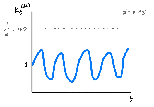
Note that \(C_t\) defined in \((1)\) is incorrect only if it excludes \(\mu\), which happens when \(K_t^{(\mu)} \geq 1/\alpha\). But this happens with probability \(\leq \alpha\) according to \((2)\). In other words, with high probability, \(C_t\) contains \(\mu\).

Figure 1: The payout rarely goes above \(1/\alpha\).
So how should we bet?
So far we haven’t discussed how we should actually bet (i.e., choose \(\lambda_t^{(m)}\)). One method is called growth rate adaptive to the particular alternative (GRAPA; Waudby-Smith and Ramdas 2024). We choose
The main issue with evaluating the above \(\lambda_t^{(m)}\) is that we don’t know \(P\). But let’s just blindly differentiate through the expectation:
The denominator begs for a Taylor expansion:
Rearranging to solve for \(\lambda^*\), we have
where we use the plug-in empirical estimates for \(\hat{\mu}_t\) and \(\hat{\sigma}_t^2\) computed from the first \(t-1\) samples.
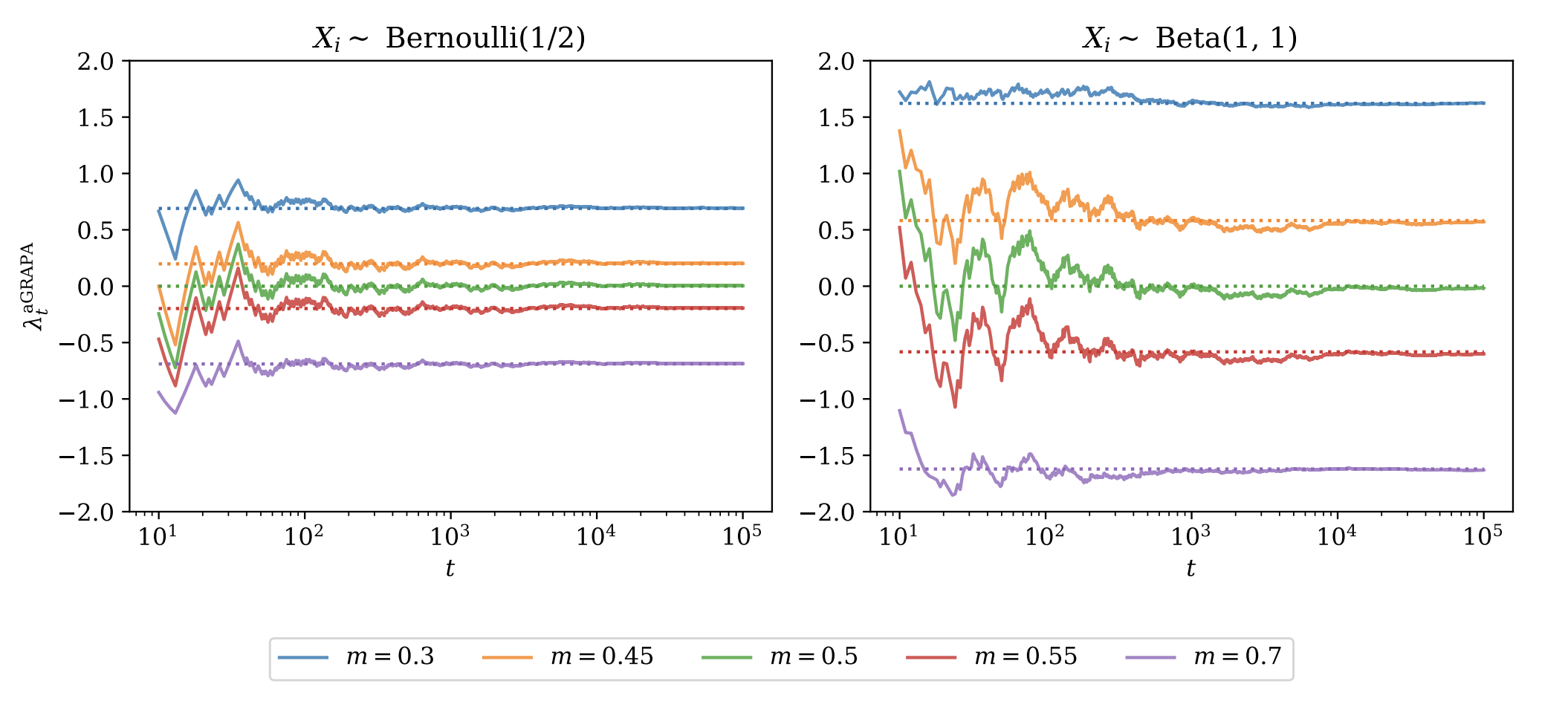
Figure 2 plots the GRAPA-chosen \(\lambda_t^{(m)}\) for five different values of \(m\), for the Bernoulli(1/2) and the Beta(1, 1) distributions. The dotted lines are “oracle” bets, where the plug-in empirical estimates \(\hat{\mu}, \hat{\sigma}^2\) have been replaced with their true values. Over time, bets converge to their oracle values.
Let’s focus on the left panel. The truth is \(\mu=0.5\), so when \(m=0.5\) (green), we see that the bet quickly converges to zero, because there is no advantage to betting. When \(m>0.5\) (\(m<0.5\)), on the other hand, the bet converges to a negative (positive) value. The absolute values of the bets become more aggressive as you are betting against values that are farther from the truth.
Beta(1, 1) on the right panel has the same mean of 0.5 but lower variance than Bernoulli(1/2). Accordingly, the bets are more aggressive on the whole.

Figure 2: Figure 10 from Waudby-Smith and Ramdas 2024
What about other estimators?
The setup presented above seems very contrived for the mean estimator. Let’s consider another estimator, the univariate M-estimator,
for some “nice” loss function \(L\).* Our payout will look like
Now \(K_t^{(\theta^*)}\) is a non-negative martingale with an initial value of 1. The arguments for non-negative and initial value 1 are the same as above, and it’s a martingale, because
where the underbrace equality holds because \(\theta^*\) is the minimizer of the expected loss, so \(\nabla_\theta \mathbb{E}_P [L(X_i, \theta^*)] = 0 \implies \mathbb{E}_P [\nabla_\theta L(X_i, \theta^*)] = 0.\) We can then write down the betting strategy similarly as \((3)\):
Following the GRAPA derivation of differentiating through the expectation and taking the Taylor approximation, we obtain
where we again use the plug-in empirical estimate using the first \(t-1\) samples, this time for the expected gradient of the loss. Based on the intuition we took away from the GRAPA figure, this result makes sense. If \(P\) is lower-variance, like the Beta(1, 1) distribution, the numerator will be smaller and the bets \(\lambda_t^{(\theta)}\) will become more aggressive.
Acknowledgments
A huge thank you to Aaditya Ramdas for the great lecture series and textbook on e-values. I also thank Clara Wong-Fannjiang for foraying into e-values with me in our aptly named (in our opinion) reading group, “Great Expectations.”
\(*\) A sufficient condition for “niceness” being that \(X\) is regular and \(\int \mathbb{E}_P[\mid \nabla_\theta L(X, \theta) \mid]\) is finite, by Fubini
References
[1] Waudby-Smith, I. & Ramdas, A. (2024). Estimating means of bounded random variables by betting. JRSS Series B: Statistical Methodology, 86(1), 1-27.
