Shapes of conformal sets in high dimensions

I became curious about the shapes of multivariate conformal regions when working on Semiparametric conformal prediction (AISTATS 2025) [1]. Included as a baseline in this paper is a simple way to extend conformal prediction to multiple response variables: to define a scalar non-conformity score.

If you are not familiar with conformal prediction, let’s briefly review the conformal calibration procedure for a single response variable (\(d=1\)). Suppose we have a point (uncalibrated) predictor \(\hat f: \mathcal{X} \to \mathbb{R}\) and an exchangeable calibration set \(\{(x^{(i)}, y^{(i)})\}_{i=1}^n\). We define a non-conformity score \(V(x, y, \hat f)\) which says how “strange” the prediction \(\hat f(x)\) is relative to \(y\). One simple example is the absolute residual \(V(x, y, \hat f) = |y - \hat f(x)|\). We evaluate this score on the calibration set to obtain a set of \(n\) scores. Then, given a user-specified miscoverage rate of \(\alpha\), we compute the empirical \(1-\alpha\) quantile of the scores. This quantile, which we denote \(q_\alpha\), sets the width of the conformal prediction interval for a test point \(x^*\), defined by

For the absolute residual, this is simply the interval \([\hat f(x) - q, \hat f(x) + q]\). Provided that the test instances are exchangeable with the calibration ones, this set is guaranteed to cover the truth \(y^*\) with probability at least \(1-\alpha\).

Now, when the response variable takes values in \(\mathbb{R}^d\) for \(d>1\), we can define a scalar non-conformity score by taking the norm of the signed error vector \(y - \hat f(x) \in \mathbb{R}^d\). That is, we generalize the score to

where \(||\cdot||_p\) indicates the \(p\)-norm. The rest of the procedure proceeds the same way, by computing the empirical \(1-\alpha\)-quantile \(q_p\) of the scalarized scores and constructing the prediction region as in Equation \(\text{(1)}\) with \(q=q_p\). There are “smarter” ways to do the scalarization, by first transforming the score space, for instance [2], but we focus on simple \(L_p\)-norm scalarizations here.

The \(\geq 1-\alpha\) coverage requirement is trivially satisfied by just returning the entire space \(\mathbb{R}^d\) as the prediction set, which would not be useful. The smaller the size (or the hypervolume in \(d\) dimensions) of the prediction set, the better in the sense that it’s more precise. This post is about how to choose \(p\) such that precision is maximized (i.e., the hypervolume of the prediction set is minimized).

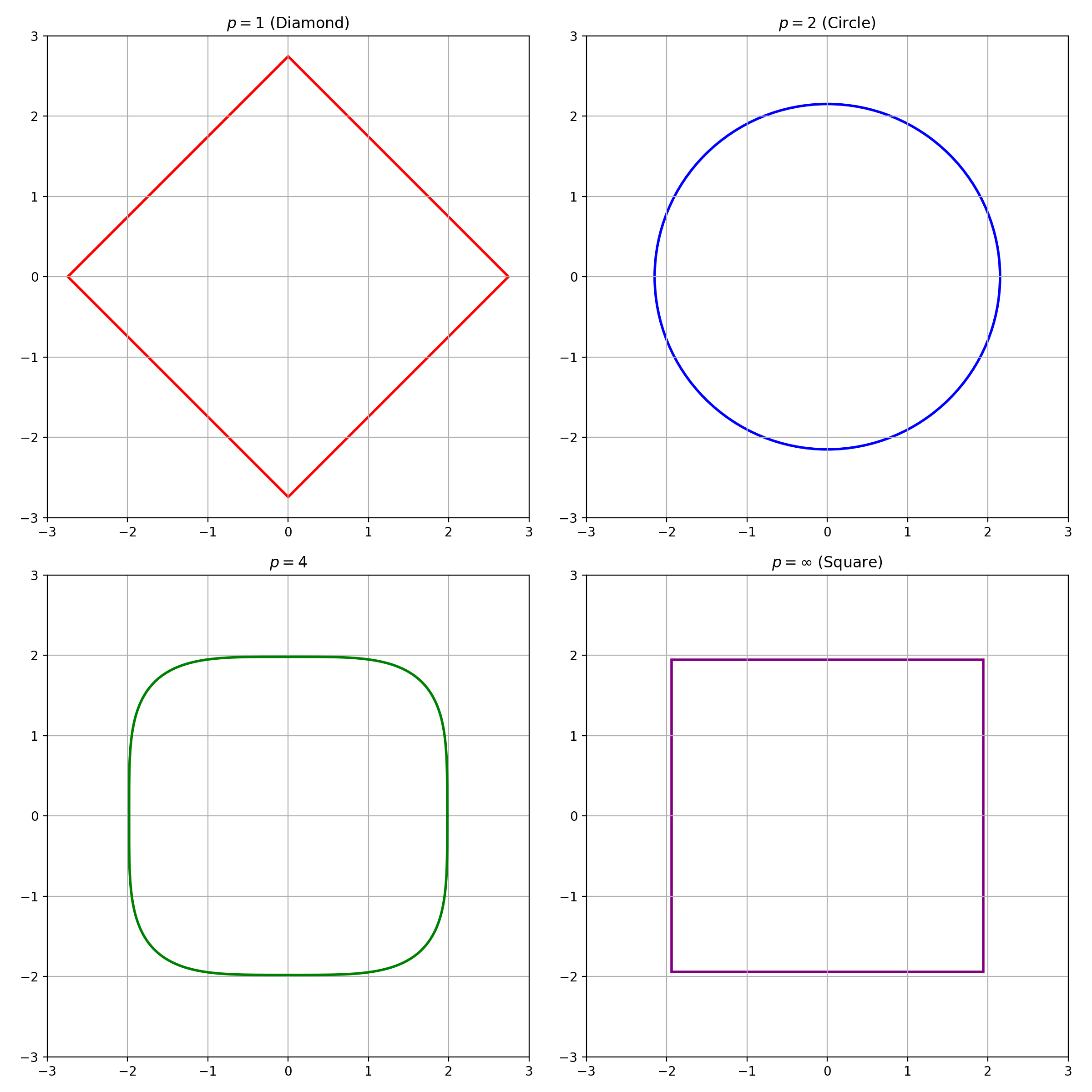
As Equation \(\text{(1)}\) suggests, shapes of prediction regions in \(d\) dimensions using the \(L_p\) norm of \(y - \hat f(x)\) as the non-conformity score are \(p\)-norm balls,

with radius \(a=q_p\) and centered at the original prediction \(\hat f(x)\). For \(d=2\), the \(L_1\) norm for the scalar score in Equation \(\text{(2)}\) yields a diamond-shaped prediction region with distance \(q_1\) from center to the corner, with area \(2 q_1^2\). The \(L_2\) norm yields a circle with radius \(q_2\), which has area \(\pi q_2^2\). The \(L_\infty\) norm yields a square with side length \(2 q_\infty\), which has area \(4 q_\infty^2\). The shapes for \(d=2\) and \(p=1, 2, 4, \infty\) look like the below, assuming \(y - \hat f(x) \sim \mathcal{N}(0, I_2)\).

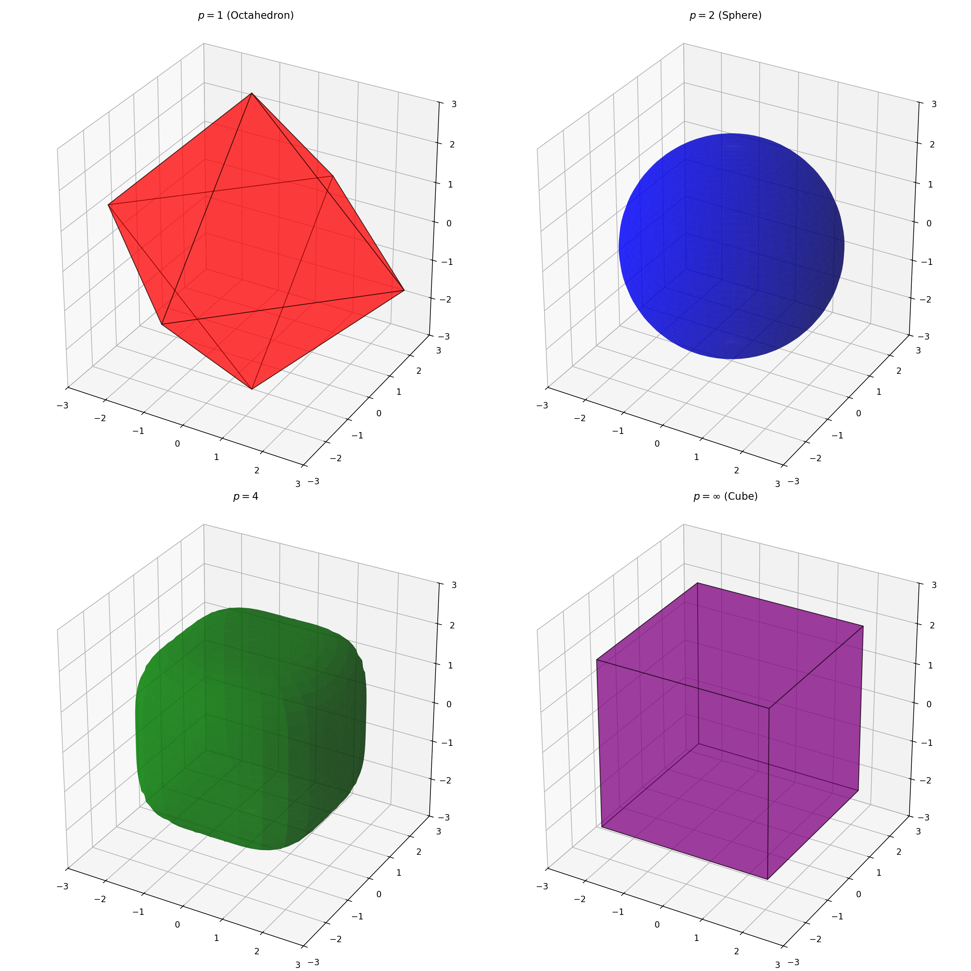
Similarly, for \(d=3\), the \(L_1\) norm for the scalar score yields a cross polytope with distance \(q_1\) from center to the corner, which has volume \(\frac{2^d}{d!}\). The \(L_2\) norm yields a ball with radius \(q_2\), which has volume \(\frac{4 }{3} \pi q_2^3\). The \(L_\infty\) norm yields a hypercube with side length \(2 q_\infty\), which has volume \(8 q_\infty^3\). The shapes for \(d=3\) and \(p=1, 2, 4, \infty\) look like the below, assuming \(y - \hat f(x) \sim \mathcal{N}(0, I_3)\).

The general formula for the (hyper)volume of a \(d\)-dimensional \(p\)-ball of radius \(a\) in Equation \(\text{(3)}\) is

The radius \(a\) to use is the quantile, \(q_p\), of the \(L_p\)-scalarized scores. This leads one to wonder if, given a distribution of signed error vectors \(y - \hat f(x)\) in \(\mathbb{R}^d\), it’s possible to “win” some precision by choosing \(p\) that gives the smallest \({\rm Vol} \left(B_p(q_p) \right)\). One observation is that, while \({\rm Vol} \left(B_p(a) \right)\) increases with \(p\) for a fixed radius \(a\), the quantile value \(q_p\) decreases monotonically with \(p\), since \(||y||_{p_1} \geq ||y||_{p_2}\) for \(p_1 \leq p_2\).

Recalling that \(q_p\) is the \(1-\alpha\) quantile of the \(p\)-norm of signed error vectors \(y - \hat f(x)\), we know that its value must depend on the distribution of the errors. For simplicitly, let us assume the errors are independent across the \(d\) response variables, and consider ones that are distributed according to the radially symmetric density

which is Gaussian when \(p^*=2\).

Given this error distribution, what is the optimal \(p\) to choose? In other words, what is the \(p\) that would yield the minimum \({\rm Vol} \left(B_p(q_p) \right)\), where \(q_p\) is the \(1-\alpha\) quantile of the \(p\)-norm of the errors?

The answer is \(p^*\) – proof to follow. This means that you can inspect the distribution of errors, specifically the slope of its density, and match the order \(p\) of the scalarizing norm. If the errors are approximately Gaussian, use their \(L_2\) norm as the non-conformity score. If they are Laplace, use the \(L_1\) norm. The radially symmetric density assumes that the scales of errors are the same across the \(d\) response variables, but the logic of the proof extends to settings with differing scales, such as ones where a response variable is particularly difficult to predict. In fact, up to monotone transformations, it applies to general convex \(r(z)\) associated with a log-concave density \(f(z) \propto e^{-r(z)}\). The result can be understood in terms of the isoperimetric inequality applied to log-concave densities [3]; for any other \(p \neq p^*\), the geometry of the \(p\)-ball is misaligned with the level sets of the density \(f\), so we pay a penalty in volume. Basically, the best scalarizing scheme is one that matches the shape of the error distribution.

We want to show that, for a random variable \(Z\) distributed according to the density \(f(z) = C e^{-||z||_{p^*}^{p^*}}\) for some constant \(C > 0\), the volume \({\rm Vol} \left(B_p(q_p) \right)\) in Equation \(\text{(4)}\) with radius \(q_p\) chosen to satisfy

is minimized if and only if \(p = p^*\).

The proof essentially depends on a well-known result that states that, for any density \(f(z)\), among all measurable sets \(A\) satisfying \(\int_A f(z) dz = 1-\alpha,\) the set that minimizes the hypervolume (the Lebesgue measure) is the highest-density region, or the superlevel set \(A^* = \{z \in \mathbb{R}^d: f(z) \geq k \}\) where \(k\) is chosen so that \(A^*\) contains mass \(1-\alpha\).

First, consider the set,

where \(r_{p^*}\) is chosen to satisfy \(\int_{B_{p^*}(r_{p^*})} f(z) dz = 1-\alpha\). This is a highest-density region, because \(||z||_{p^*} \leq r_{p^*} \iff f(z) \geq C e^{-r_{p^*}}\). This means that, for any other measurable set \(A\) satisfying \(\int_A f(z) dz = 1-\alpha\), we have \({\rm Vol} \left( B_{p^*}(r_{p^*}) \right) \leq {\rm Vol}(A)\). This includes sets of the form \(B_p(q_p)\) with \(q_p\) chosen to satisfy \(\int_{B_p(q_p)} f(z) dz = 1-\alpha\). The minimum volume for \(B_p(q_p)\) occurs at \(p = p^*\).

References

[1] Park, Ji Won, Robert Tibshirani, and Kyunghyun Cho. “Semiparametric conformal prediction.” AISTATS (2025).

[2] Feldman, Shai, Stephen Bates, and Yaniv Romano. “Calibrated multiple-output quantile regression with representation learning.” JMLR (2023).

[3] Bobkov, S.G. “Isoperimetric and Analytic Inequalities for Log-Concave Probability Measures.” Annals of Probability (1999).