What we talk about when we talk about influence functions: Part 2

In Part 1 of this series, we showed that the efficient influence function (EIF) coincides with the leave-one-out empirical influence function (EmpIF) in finite samples if the underlying distribution is the empirical distribution and the estimand is the mean estimand.

Being a linear estimator, the mean \(\Psi(P) = \mathbb{E}_P[X]\) is a “nice” estimand. This means that it’s a linear functional of the distribution. That is, for any pair of distributions \(P, Q\) and any \(\alpha \in [0, 1]\), a linear functional \(\Psi\) satisfies \[\Psi\left(\alpha P + (1-\alpha) Q \right) = \alpha \Psi(P) + (1-\alpha)\Psi(Q).\]

Quantile functionals: the EIF

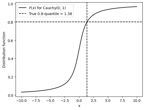
Now let’s consider a non-linear functional, the quantile. For this post, we will be identifying measures \(P\) with their distribution functions \(F\), for notational simplicity. The functional \(\Psi\) will thus take as its argument the distribution function \(F\) associated with \(P\), rather than \(P\) itself. The \(\tau\)-quantile estimand (quantile at level \(\tau\)) can be implicitly defined as \(\Psi_\tau(F)\) satisfying \[F\left( \Psi_\tau(F) \right) = \tau.\]Equivalently, we may write it in terms of the quantile function \(F^{-1}\): \[\Psi_\tau(F) = F^{-1}(\tau).\] As an example, let’s take the Cauchy distribution. The true distribution function \(F\) is the solid black curve, and the true quantile \(\Psi(F)\) in dashed black is where the distribution function equals \(\tau=0.8\).

We will derive EIF like we did in Part 1. First, note that the quantile can be implicitly written in terms of the probability density function (PDF) \(f\): \[\int_{-\infty}^{\Psi_\tau(F)} f(s) ds = \tau.\] The \(\delta\)-contaminated density that we associate with the \(\delta\)-contaminated distribution \(F_\epsilon\) is then \(f_\epsilon(s) = (1-\epsilon)f(s) + \epsilon \delta_x(s)\), where we have contaminated the original density \(f(s)\) with a Dirac measure located at \(x\), a measure assigning probability 1 to \(\{x\}\) and 0 to all other elements in \(\mathbb{R}\). For this density, \[\int_{-\infty}^{\Psi_\tau(F)} f_\epsilon(s) ds = \tau. \tag{1}\] Recall that EIF can then be derived as the following generalized derivative:\[{\rm EIF} \equiv \psi(x; F, \Psi) = \lim_{\epsilon \to 0} \frac{\Psi_\tau(F_\epsilon) - \Psi_\tau(F)}{\epsilon}.\] Now differentiating both sides of \((1)\) with respect to \(\epsilon\) using the Leibniz integral rule,

Rearranging,

The integrand is \[\frac{d f_\epsilon(s)}{d \epsilon} = -f(s) + \delta_x(s),\] and note that \(\int_{-\infty}^{c} f(s) ds = F(c)\) and \(\int_{-\infty}^{c'} \delta_x(s) ds = 1[x \leq c']\), where \(1[\cdot]\) is the indicator function, for \(c, c' \in \mathbb{R}\). Finally, then, we have

Evaluating at \(\epsilon=0\), we have derived the EIF:

In the numerator, you may recognize the derivative of the pinball loss used for quantile regression. The pinball loss is \(l_\tau(x) = x\left(1[x \geq 0] - (1-\tau)\right)\), and its derivative \(l'_\tau(x) = 1[x \geq 0] - (1-\tau).\)

Quantile functionals: the EmpIF

Similarly as for the mean estimand, the leave-one-out EmpIF can be written as the (scaled) difference: \[{\rm EmpIF} = \psi_{\rm emp}(x_j; \Psi_\tau) = (n-1)\left(\Psi_\tau(F_n) - \Psi_\tau\left(F_n^{-j}\right)\right), \tag{2}\]where \(F_n\) is the distribution associated with the empirical measure \(P_n\) and \(F_n^{-j}\) is the distribution with the \(j\)-th data point \(x_j\) removed.

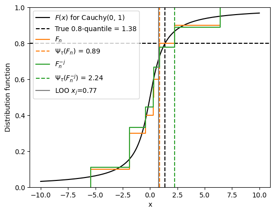
Going back to the Cauchy example, suppose we draw 20 samples from this distribution, yielding the empirical distribution \(F_n\) in orange and its empirical quantile, \(\Psi_\tau(F_n) = 0.89\). We remove one data point, \(x_j\), and obtain the green distribution \(F_n^{-j}\), in green and its empirical quantile, \(\Psi_\tau(F_n^{-j}) = 2.24\). Because \(x_j\) is relatively small, the quantile estimate goes up when we remove it.

Recall that, in Part 1, where we discussed the mean functional, the leave-one-out EmpIF \(\psi_\textrm{emp}(x_j; \Psi_\tau)\) was equal to the EIF evaluated at the empirical measure, \(\psi(x; F_n, \Psi_\tau)\). We will now show that the equality does not hold with the quantile functional \(\Psi_\tau\). In fact, \(\psi_\textrm{emp}(x_j; \Psi_\tau)\) and \(\psi(x; F_n, \Psi_\tau)\) only coincide in the large \(n\) limit.

Let’s first relate the two terms that enter the difference in Equation \((2)\). The full-sample distribution is \[F_n(t) = \frac{1}{n} \sum_{i=1}^n 1\left[ x_j \leq t \right],\] whereas the distribution with \(x_j\) left out is \[F_n^{-j}(t) = \frac{1}{n-1} \sum_{i \neq j} 1\left[ x_i \leq t \right].\] These are related by \[F_n^{-j}(t) = \frac{1}{n-1} \left( n F_n(t) - 1 \left[x_j \leq t \right] \right).\] When \(t=\Psi_\tau (F_n)\), \[F_n^{-j}\left( \Psi_\tau (F_n) \right) = \frac{n}{n-1} \tau - \frac{1}{n-1} 1 \left[x_j \leq \Psi_\tau (F_n) \right], \tag{3}\] using the fact that \(F_n(\Psi_\tau(F_n)) = \tau\).

Next, let us consider the true distribution \(F\) and for notational simplicity define \(q^{-j} \equiv \Psi_\tau(F_n^{-j})\) and \(q = \Psi_\tau(F_n)\). Since \(q^{-j}\) and \(q\) are close together, we can Taylor-expand \(F(q^{-j})\) around \(q\). Setting \(\Delta \equiv q^{-j} - q\), we have \[F(q^{-j}) = F(q) + f(q) \Delta + \frac{1}{2} f’(q) \Delta^2 + \mathcal{O}\left(\Delta^3 \right),\] where \(f\) is the density function associated with \(F\) and \(f'\) is its derivative.

The leave-one-out EmpIF in Equation \((2)\) is \(-(n-1)\Delta\), so let’s solve for \(\Delta\). Rearranging the above, \[\Delta + \frac{1}{2} \frac{f’(q)}{f(q)} \Delta^2 + \mathcal{O}\left(\Delta^3 \right) = \frac{F(q^{-j}) - F(q)}{f(q)}.\] Here, we will wave hands a little bit and now substitute \(F^{-j}_n\) for \(F\) on the RHS. We are justified in doing so for asymptotic analysis, because \(F_n^{-j}\) approaches \(F\) in the large-\(n\) limit. We now have

The leading-order term is \(\Delta_1\), so let us express \(\Delta\) as this plus a second-order correction — that is, \(\Delta \equiv \Delta_1 + \Delta_2\). We already know what this leading term \(\Delta_1\) looks like. In the numerator, \(F^{-j}_n(q^{-j})\) is simply \(\tau\) and we already worked out the second term in Equation \((3)\). \[\Delta_1 = \frac{1}{f(q)} \left( \tau - \frac{n}{n-1} \tau + \frac{1}{n-1} 1 \left[x_j \leq \Psi_\tau (F_n) \right] \right) = \frac{1}{n-1} \times \frac{1\left[x_j \leq \Psi_\tau(F_n) \right] - \tau}{f(q)}\] Almost there. Canceling terms in Equation \((4)\), the second-order term is then \[\Delta_2 = -\frac{1}{2} \frac{f’(q)}{f(q)} \Delta_1^2 + \mathcal{O}\left(n^{-3} \right).\] Finally, the leave-one-out EmpIF is

So we have recovered the EIF, evaluated at the empirical measure, as the first term. There are some remainder terms that arise because the quantile functional is not linear in the underlying measure.

Numerical verification

Let’s evaluate the EIF with the true population quantile, EIF with the empirical quantile, and the leave-one-out EmpIF and see how they compare with increasing \(n\).

np.random.seed(42)

# We will use the Cauchy distribution as an example,
# since it has an analytical quantile function

dist_obj = stats.cauchy(loc=0, scale=1)
tau = 0.8 # target quantile level
sample_sizes = np.logspace(1, 3, 10).astype(int)
num_trials = 100

# Init arrays to store results
eif = np.empty((num_trials, len(sample_sizes)))
eif_true = np.empty((num_trials, len(sample_sizes)))
empif = np.empty((num_trials, len(sample_sizes)))

def get_eif_quantile_cauchy(x, tau, dist_obj, plug_in_quantile):
"""Evaluate efficient influence function with the empirical quantile"""
    return (tau - (x <= plug_in_quantile).astype(float))/dist_obj.pdf(plug_in_quantile)

  
def get_true_eif_quantile_cauchy(x, tau, dist_obj):
"""Evaluate efficient influence function with the true quantile"""
    true_quantile = dist_obj.ppf(tau)
    return (tau - (x <= true_quantile).astype(float))/dist_obj.pdf(true_quantile)


for i in range(num_trials):
    for j, num_samples in enumerate(sample_sizes):
		samples = dist_obj.rvs(size=num_samples)
		# Compute Psi(F_n), Psi(F_n^{-j})
		query_j = np.random.choice(num_samples) # chose leave-one-out index
		samples_minus_j = np.delete(samples, query_j)
		empirical_tau_quantile = np.quantile(samples, tau, method="inverted_cdf")
		empirical_tau_quantile_minus_j = np.quantile(samples_minus_j, tau, method="inverted_cdf")
		# Compute EIF with empirical quantile and true quantile
		eif[i, j] = get_eif_quantile_cauchy(samples[query_j], tau, dist_obj, empirical_tau_quantile)
		eif_true[i, j] = get_true_eif_quantile_cauchy(samples[query_j], tau, dist_obj)
		# Compute leave-one-out EmpIF
		empif_val = (empirical_tau_quantile - empirical_tau_quantile_minus_j)*(num_samples-1)
		empif[i, j] = empif_val

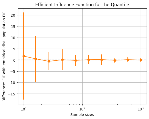
As expected, the population EIF and EIF evaluated using the empirical quantile coincide as \(n\) increases, as the empirical quantile approaches the true quantile.

diff = eif - eif_true
plt.errorbar(sample_sizes, diff.mean(0), yerr=diff.std(0), marker="o", color="tab:orange")
plt.axhline(0, linestyle="--", color="k")
plt.xlabel("Sample sizes")
plt.ylabel("Difference: EIF with empirical dist - population EIF")
plt.title("Efficient Influence Function for the Quantile")
plt.grid(True)
plt.xscale("log")

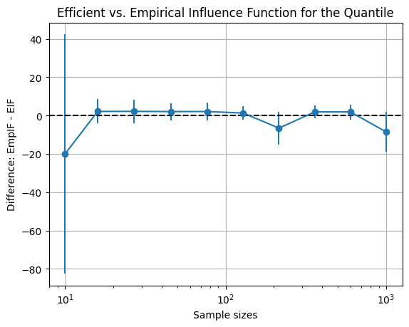
The leave-one-out EmpIF, on the other hand, carries more finite-sample variance.

diff = empif - eif
plt.errorbar(sample_sizes, diff.mean(0), yerr=diff.std(axis=0), fmt='o-')
plt.axhline(0, linestyle="--", color="k")
plt.xlabel("Sample sizes")
plt.ylabel("Difference: EmpIF - EIF")
plt.title("Efficient vs. Empirical Influence Function for the Quantile")
plt.grid(True)
plt.xscale("log")

Today, we focused on comparing the EIF (evaluated at the empirical measure) with the leave-one-out EmpIF. The quantile was a simple example of a non-linear functional that didn’t involve fitting a model. One model-specific example of key interest to robust statistics and ML interpretability is the M-estimator: \[\Psi(P) \equiv \arg \min_\theta \ \mathbb{E}_{X \sim P} [ G(X, \theta)],\] where \(G(X, \theta)\) is some per-instance loss function. It can be, for instance, the loss function of a model parameterized by \(\theta\) with respect to a training instance \(X\). Because leave-one-out retraining for every single training instance is unfeasible, the EIF provides a cheap approximation under some assumptions, including a strongly convex loss landscape. When these assumptions are violated, as they are with nonlinear neural networks, it can be very fragile. See Basu et al. (2020) and Bae et al. (2022).

Part 3 will be dedicated to the EIF and its relevance to semiparametric efficiency theory.

References

[1] Basu, S., Pope, P., & Feizi, S. (2020). Influence functions in deep learning are fragile. ICLR.

[2] Bae, J., Ng, N., Lo, A., Ghassemi, M., & Grosse, R. B. (2022). If influence functions are the answer, then what is the question?. NeurIPS.